Behind the Scenes: AI Image Generation
In this post we are going to take a look at how image generation models work and their evolution.
Pre-VAE and GAN Era
There were several approaches to image generations before VAE and GANs. While they were able to lay the groundwork for VAE and GANs, they lacked scalability and quality of VAE or GAN generated images. Here we quickly review some of the approaches and the key idea behind them.
- Principal Component Analysis(PCA): PCA can be used in generative scenarios. One could sample from the the original components and then reconstruct the approximate input. $x = Wz + \mu$ where $z \sim \mathcal{N}(0, I)$. In order to generate new images, one could sample from the latent space and then transform it into the data space. This approach is very fast, however, it has a very poor sample diversity. [1]
- Independent Component Analysis(ICA): ICA is similar to PCA but it enforces sparsity or independence in latent space. Like PCA, one would sample from the latent space $x = Wz$ and then reconstruct the approximate input. It encourages features like edge detector, however, it acts like a fixed dictionary and has no learned decoder. [2]
- Classical Autoencoders: $ x \rightarrow z \rightarrow \hat{x} $ where $z$ is a latent variable and $\hat{x}$ is the reconstructed input. Neural networks are utilized in order to reconstruct the input. The downside of this approach is that you cannot reliably sample random points. There is no real generative process. [3]
- Restricted Boltzman Machines(RBM) and Deep Belief Networks(DBN): Both of them relied on energy-based models. They could be considered true early generative models. They are able to generate images, however, they are not able to generate high quality images. Their main limitations were both sampling and training time was very slow. [4,5,6]
Introduced in 2013, Variational Autoencoders(VAEs) [7] combines ideas from probability and neural networks. Here are the key ideas introduced in this paper:
- They assume that the data is generated from latent variables and use probabilistic framework in order to train neural encoder and decoder.
- Introducing reparameterization trick which enables differential sampling from latent variables. This in turn will allow backpropagation through stochastic layers. Previously it wasn’t possible to train latent variable models via stochastic gradient descent (SGD).
- Variational inference was hard to scale previously. Instead they introduced Gradient Variational Bayes (SGVB) which made it possible to train variational models on large datasets via minibatch.
Here is how the basic math works for VAEs. VAEs try to model a generative process where:
- Sample latent variable $z \sim p(z)$.
- Generate data $x \sim p_{\theta}(x\mid z)$.
But the posterior $p(z\mid x)$ is intractable, meaning, it cannot be computed efficiently or in closed form. As a result, we use a neural encoder, $q_{\phi}(z\mid x)$, to approximate it.

The intuition is that the encoder tries to map $x$ to a distribution over latent space $z$. The decoder tries to map $z$ back to a distribution over data space $x$.
Post-training, VAEs consist of two parts:
- Encoder, $q_{\phi}(z\mid x)$, that maps input image ($x$) to a distribution over latent space ($z$).
- Decoder, $p_{\theta}(x\mid z)$, that maps latent space ($z$) to a distribution over data space ($x$).
For generation, only the decoder is used and the encoder is not used.
- Sample $z$ from a prior distribution $p(z)$. E.g. $z \sim \mathcal{N}(0, 1)$. This becomes the start token in a way.
- Decoder is used to generate image $\hat{x} = p_{\theta}(x\mid z)$.
- The decoder output could be image, probability distribution over words/tokens, or a waveform.
Aside from image generation use cases of VAEs, one interesting application of VAE’s latent variables is to use them for encoding information and then later on use them for similarity search or clustering.
Generative Adversarial Network(GAN) [8] was introduced in 2014. The core idea behind this paper is using some form of game theoretic setup. There are two models that are being trained simultaneously, Generator(G) and Discriminator(D). The goal of generator is to generate realistic image and the goal discriminator is tell whether an image was generated by the model or it’s a real image. Both models iteratively improve. Unlike earlier versions of generative models, GANs, don’t use sampling or compute likelihoods and instead rely on backpropagation which makes the training computationally straightforward.
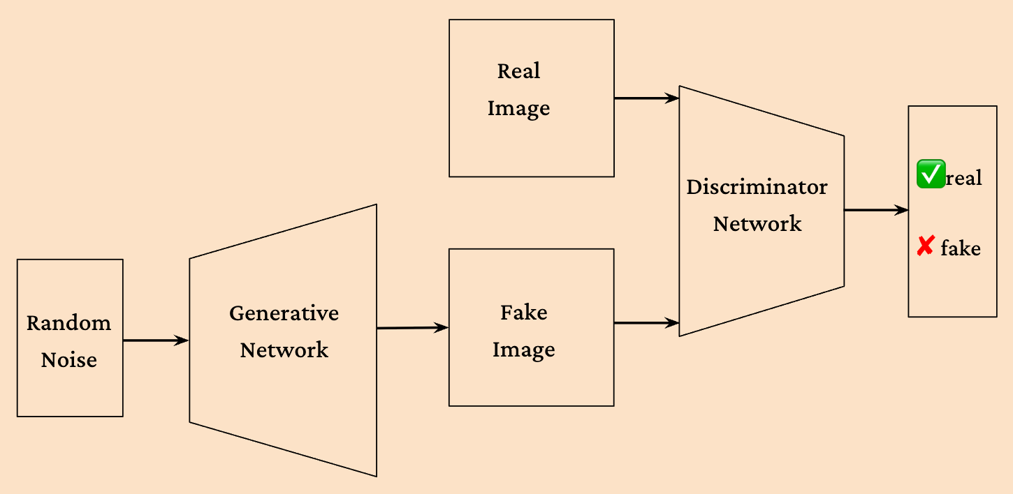
- In the discrimination phase, we want D to have the following behavior:
- In the generation phase, we want G to have the following behavior:
As a result, our objective function for training D and G becomes:
Discrimination phase: \(\max \nabla_{\theta_{d}} \frac{1}{m} \sum_{i=1}^{m} [logD(x_i) + log(1-D(G(z_i)))]\)
Generation phase: \(\min \nabla_{\theta_{g}} \frac{1}{m} \sum_{i=1}^{m} log(1-D(G(z_i)))\)
Note that in Tensorflow and other frameworks, since we would like to work with minimization objective functions and also positive loss values, the above objective functions are turned into:
Discrimination phase: \(\max \nabla_{\theta_{d}} \frac{1}{m} \sum_{i=1}^{m} [-logD(x_i) - log(1-D(G(z_i)))]\)
Generation phase: \(\min \nabla_{\theta_{g}} \frac{1}{m} \sum_{i=1}^{m} [-log(D(G(z_i)))]\)
GANs turned out to be very powerful and scalable and a plethora of new versions of GANs introduced in the years following the original paper. Here are some of the most notable ones:
Conditional GANs(2014): Conditional GANs. [9]
This paper was published soon after the original GAN paper. In this paper, they simply added a class label to both the generator and the discriminator. This class label is the condition that the generator and discriminator should be conditioned on. For example, by passing the class label to the generator, it will generate an image of that class. This paper lead to a lot of other cool GAN research papers such as Pix2Pix, StyleGAN3, text-to-image GANs.
DCGANs(2015): Deep Convolutional GANs. [10]
By using proper architecture and replacing the fully connected layers with convolutional layers, they achieved stable training.
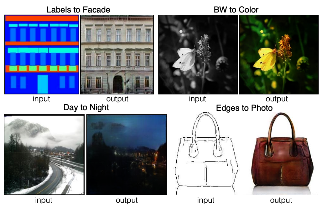
Pix2Pix (2016): [11] This paper took the idea of conditional GANs and applied it to image-to-image translation. The idea is that you have a source image and a target image. You want to learn a mapping from the source image to the target image. In order to achieve this goal, L1 + adversarial loss is used.
Wasserstein GAN(2017): [12]
This work replaced the original GAN loss with a Wasserstein loss. This lead to a much more stable training and better convergence.
StyleGAN Series (2019–2021): [13, 14, 15] In style GAN series, they separated the latent space from the image features. Instead of inputting the $z$ directly to the generator, they input $z$ and a learned style code $w$. This decoupling of the latent space from the image features allows for more control over the generated image. They also injected style at different layers of the generator. Early layers control pose and layout and later layers control texture and color. Middle layers control the overall structure of the image. The image generated by style GANs showed unprecedented quality. StyleGAN2 was particularly a successful work in this series since it introduced:
- High-quality image generation.
- Semantic control via latent space.
- Much more stable training.

StyleGAN was the peak of the GAN era. It provided unprecedented quality in image generation. 2020 marks the beginning of the diffusion era where the focus shifted to diffusion models. Diffusion models were able to address limitations of GANs such as:
- Showed better sample quality, more diversity, and fewer training instabilities.
- GANs struggled with complex conditioning like free form text. However, diffusion models integrated easily with language models such as CLIP.
- No major architectural breakthroughs in GANs.
- Diffusion models did better by scaling data and compute and research labs gradually shifted their focus to diffusion and transformer models.
References:
- Michael E. Tipping, Christopher M. Bishop, Probabilistic Principal Component Analysis, Journal of the Royal Statistical Society Series B: Statistical Methodology, Volume 61, Issue 3, September 1999, Pages 611–622, https://doi.org/10.1111/1467-9868.00196
- Comon, P. (1994). Independent component analysis, A new concept? Signal Processing, 36(3), 287–314. https://hal.science/hal-00417283v1/file/como94-SP%20%281%29.pdf
- Hinton, G. E., & Salakhutdinov, R. R. (2006). Reducing the dimensionality of data with neural networks. Science, 313(5786), 504–507. https://science.sciencemag.org/content/313/5786/504
- Hinton, G. E., Osindero, S., & Teh, Y.-W. (2006). A fast learning algorithm for deep belief nets. Neural Computation, 18(7), 1527–1554. https://doi.org/10.1162/neco.2006.18.7.1527
- Hinton, G. E., Osindero, S., & Teh, Y.-W. (2006). A fast learning algorithm for deep belief nets. Neural Computation, 18(7), 1527–1554. https://doi.org/10.1162/neco.2006.18.7.1527
- Hinton, G. E., & Salakhutdinov, R. R. (2006). Reducing the dimensionality of data with neural networks. Science, 313(5786), 504–507. https://doi.org/10.1126/science.1127647
- Kingma, D.P., Welling, M. (2013). Auto-Encoding Variational Bayes. arXiv preprint arXiv:1312.6114. https://arxiv.org/abs/1312.6114
- Goodfellow, I.J., Pouget-Abadie, J., Mirza, M., Xu, B., Warde-Farley, D., Ozair, S., Courville, A., Bengio, Y. (2014). Generative Adversarial Networks. arXiv preprint arXiv:1406.2661. https://arxiv.org/abs/1406.2661
- Mirza, M., Osindero, S. (2014). Conditional Generative Adversarial Nets. arXiv preprint arXiv:1411.1784. https://arxiv.org/abs/1411.1784
- Radford, A., Metz, L., Chintala, S. (2015). Unsupervised Representation Learning with Deep Convolutional Generative Adversarial Networks. arXiv preprint arXiv:1511.06434. https://arxiv.org/abs/1511.06434
- Isola, P., Zhu, J., Zhou, T., Efros, A.A. (2016). Image-to-Image Translation with Conditional Adversarial Networks. arXiv preprint arXiv:1611.07004. https://arxiv.org/abs/1611.07004
- Arjovsky, M., Chintala, S., Bottou, L. (2017). Wasserstein GAN. arXiv preprint arXiv:1701.07875. https://arxiv.org/abs/1701.07875
- Karras, T., Laine, S., Aila, T. (2018). A Style-Based Generator Architecture for Generative Adversarial Networks. arXiv preprint arXiv:1812.04948. https://arxiv.org/abs/1812.04948
- Karras, T., Laine, S., Aittala, M., Hellsten, J., Lehtinen, J., Aila, T. (2019). Analyzing and Improving the Image Quality of StyleGAN. arXiv preprint arXiv:1912.04958. https://arxiv.org/abs/1912.04958
- Karras, T., Aittala, M., Laine, S., Härkönen, E., Hellsten, J., Lehtinen, J., Aila, T. (2021). Alias-Free Generative Adversarial Networks. arXiv preprint arXiv:2106.12423. https://arxiv.org/abs/2106.12423