Introduction
Reinforcement Learning
Q-learning and Bellman Equation
Q-learning in Atari Games
Experience Replay
DQN2 Innovations
Questions
Future Works
References

Introduction

In this post I am going to talk about Deep Q Learning (DQN). The main idea is based on two papers that were published in 2013(NeurIPS) and 2015(Nature) by Google Deepmind. For the sake of simplicity, I am going to refer to these papers as DQN1 and DQN2.

DQN1: Playing Atari with Deep Reinforcement Learning¹

DQN2: Human-level Control Through Deep Reinforcement Learning²

The primary focus of these two papers is to develop a method for outperforming computers in Atari games with minimal supervision from humans. The papers combine ideas from reinforcement learning and deep learning (CNN) in order to achieve the above human level performance.

Reinforcement Learning

Before delving into the paper, let’s very briefly talk about reinforcement learning. In reinforcement learning, there is an agent that interacts with an environment(in this case gaming), takes an action, receives a reward or punishment depending on the action. In the case of the Atari game, the agents actions are moving the joysticks(in emulation) and the reward is the score that the agent receives. The goal of the agent is to maximize the reward. The agent learns by taking an action, receiving a reward, and then updating its knowledge about the environment. The knowledge about the environment is stored in a table called Q-table. Q-table consists of rows and columns. Below is a sample Q-table. In this table, rows are states and columns are the actions. And each cell in the table is the expected reward for taking an action in a given state. For example, if the agent is in state 1 and takes action 1, the expected reward is 0.1.

Sample Q-table
State	Action 1	Action 2	Action 3	Action 4
1	0.1	0.2	0.3	0.4
2	0.5	0.6	0.7	0.8
3	0.9	0.10	0.11	0.12
4	0.13	0.14	0.15	0.16

This table will get updated each time the agent plays the game or in short episodes. But how does the agent update the table? They use a method called Q-learning.

Q-learning and Bellman Equation

Q-learning is a dynamic programming approach for updating our estimation about agent’s future success. In Q-learning, agents experience consists of a sequence of distinct stages or episodes. You can think of $n$ as the number of times that agent has played the game and $t$ as the number of steps that agent has taken in a single game.

At the $t^{th}$ time step of the $n^{th}$ episode, agent:

Observes its current state $s_t$
Selects and performs an action $a_t$
Observes the subsequent state $s_{t+1}$
Adjusts its $Q_{n-1}$ value using the learning factor $\alpha_{n}$ according to the Bellman equation below:

\[Q_{n}(s_t,a) = \begin{cases} (1-\alpha_{n})Q_{n-1}(s_t,a) + \alpha_{n}[{r_t} + \gamma V_{n-1}(s_{t+1})], & \text{if not terminal state} \\ Q_{n-1}(s_t,a), & \text{if terminal state} \end{cases}\]

$V_{n-1}(s_{t+1})$ is the best possible value that the agent can achieve from state $s_{t+1}$ on ward, in other words expected future reward.

\[V_{n-1}(s_{t+1}) = \max_{a'} {Q_{n-1}(s_{t+1},{a'})}\]

$\alpha_n$ is the learning factor. It determines the balance between exploration and exploitation. Typically $\alpha_n$ is a function of $n$. During the first few episodes, $\alpha_n$ is close to $1$ and we gradually decrease it to $0$.
- If $\alpha_n = 0$, agent does not learn and exploits prior information.
- If $\alpha_n = 1$, agent learns new things and explores the environment.
$r_t$: Immediate reward received at time $t$.
$\gamma$: Discount factor, which weighs the importance of future rewards. The lesser value for $\gamma$ signifies that future rewards are less valuable and agent cares more about the immediate reward.

Q-learning in Atari Games

While updating the table seems feasible for a small number of states, in the case of Atari games, this is impractical due to the large number of states and instead we use a function approximator. In the DQN1 paper a convolutional neural network (CNN) is used to estimate the Q-table in reinforcement learning. The actual reward $r$ at each time step is provided by the simulation environment, referred to by the authors as an emulator. One thing that DQN changed is, they are using Deep CNN in order to perform the lookup. In other words, they are using CNN in order to estimate $Q$ function, i.e. CNN as a function approximator.

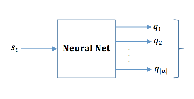
The papers combine ideas from reinforcement learning (Q-learning) and deep learning (CNN) in order to achieve the above human level performance. But you might ask, how does the Q-learning, CNN, and the table above are connected to each other? The answer is that CNN replaces the Q-table. In other words, they use the CNN in order to compute the expected utility of taking an action. Consider an agent in state $s_t$, representing the pixel images of an Atari game. They take four consecutive frames, stacking them to form $s_t$. This state is input into the CNN, which outputs various $Q$ values for each action. For instance, in a game with four possible actions, the network produces four distinct $Q$ values, each linked to an action. The action with the highest $Q$ value is recorded as $a$. This action $a$ is then input into the emulator, which returns the reward $r$ and the subsequent state $s_{t+1}$. The tuple $(s_t, a, r, s_{t+1})$ is then stored in memory.

Network Q

Here is the pseudo code for the algorithm:

Initialize replay memory $D$ to capacity $N$.
Initialize the neural network with random weights $\theta$, which approximates the action-value function.
For each episode $e$ from $1$ to $M$:
- Initialize sequence $s_1$. (${s_1}$ could be a sequence of frames)
- For each time step $t$ from $1$ to $T$:
  - Experience Generation
    - With probability $\epsilon$ select a random action $a_t$.
    - Otherwise, select $a_t = argmax_a CNN(s_t, a; \theta)$. Basically, pass the current state $s_t$ to CNN and it will output all possible $Q$ values. Finally, choose the one with the highest value and call it $a_t$.
    - Execute action $a_t$ in the emulator and observe reward $r_t$ and next state(image in this case) $s_{t+1}$.
    - Store transition $(s_t, a_t, r_t, s_{t+1})$ in the memory $D$. Note the randomness in selecting action $a_t$. This is coming from experience replay. We will talk about it later.
  - Training the Network
    - Sample random minibatch of transitions $(s_j, a_j, r_j, s_{j+1})$ from $D$.
    - Set target $y_{target}$ for each sampled transition:
      - If $s_{j+1}$ is terminal, then $y_{target} = r_j$. In other words, if the game is won(lost), then the target is the immediate reward(punishment).
      - If $s_{j+1}$ is non-terminal, then $y_{target} = r_j + \gamma max_{a’}CNN(s_{j+1}, a’; \theta)$. Notice the similarity between this equation and the Bellman equation for Q-learning.
    - Set prediction $y_{prediction} = CNN(s_j, a_j; \theta)$.
    - Perform a gradient descent step on $(y_{target} - y_{prediction})^2$ with respect to the network parameters $\theta$.
- End for each time step.
End for each episode.

Experience Replay

If you pay close attention to the training part in the algorithm above, the CNN is not trained based on the current state of the game. That’s why their approach is off-policy. What does this mean? It means they train the network by taking a random sample $(s_t, a, r, s_{t+1})$ from memory and not based on the current state of the game.

They are doing this for three main reasons:

Data efficiency since each sample can be used multiple times
Learning directly from consecutive samples is inefficient due to correlation between samples. This is also called autocorrelation. In other words, consecutive samples are highly correlated and can lead to divergence in parameters and unstable learning.
Experience Replay avoids diversion in parameters. The current parameters are different from those used to generate samples because samples are taken from memory not current experience. On the other hand, when learning on-policy, the current parameters determine the next data samples that parameters are trained on. For example, if the maximizing action is to move left, then training samples will be dominated by samples from left-hand side.

DQN2 Innovations

The DQN2 paper has a very similar concept to DQN1. However there are still differences such as below:

They use two different networks one for target network and another for the prediction network. The parameters of target networks are non-trainable but parameters of prediction network are trainable. At every $C$ iteration, parameters of target network are cloned from prediction network.
They also are using $\theta_{i-1}$ in the notation for $y_i$ in order to update the weights of neural network. This is a very clever approach that they use in the paper. This makes the algorithm more stable. Generating targets using an older set of parameters adds a delay between the time an update is made to $Q$ and the time update affects the target $y_j$. This will make divergence and oscillation less likely. In other words predictions are based on parameters of a few steps back rather than the parameters that just have been updated.
They add t-SNE visualization in order to show hidden representation of image frames. They show that similar image frames end up with similar 2-D representations.

Questions

Some questions that I had when I was trying to understand the algorithm:

What is the states $s$? It is raw image pixels, sequence of $k$ frames. This way we can consider temporal differences as well as being able to play roughly $k$ more times.
What is output of the neural network? Output of the neural network is the value function estimating future reward $Q_t$ for each action $a$.
What is experience reply? In short, experience reply refers to times when we don’t use the most recent observations in order to update the weights rather we sample from memory and update the weights based on this sample.
What is the target label they use in their training? Generally, in supervised learning the target value (ground truth labels) is known beforehand. However, in DQN papers the target value depends on the weights of neural network.

Future Works

As mentioned in DQN2 paper, one of the possible future areas of exploration could be choosing best memories and discarding memories that do not have sufficient information. Right now, they just override the oldest memories with the newest episodes. What could be done differently? One idea could be, after $M$ number of episodes of training, we could use t-SNE or other dimensionality reduction algorithms to remove similar memories and keep few of them instead of having a lot of similar experiences. This way we could have a more diverse set of memories.