This post is a shorter version of my longer ArXiv paper on the technical evolution of image generation models. For a full list of references please refer to the original paper.
Image generation has advanced rapidly over the past decade, yet the literature seems fragmented across different models and application domains. This paper aims to offer a comprehensive survey of breakthrough image generation models, including variational autoencoders (VAEs), generative adversarial networks (GANs), normalizing flows, autoregressive and transformer-based generators, and diffusion-based methods. We provide a detailed technical walkthrough of each model type, including their underlying objectives, architectural building blocks, and algorithmic training steps. For each model type, we present the optimization techniques as well as common failure modes and limitations. We also go over recent developments in video generation and present the research works that made it possible to go from still frames to high quality videos. Lastly, we cover the growing importance of robustness and responsible deployment of these models, including deepfake risks, detection, artifacts, and watermarking.
Variational Autoencoders
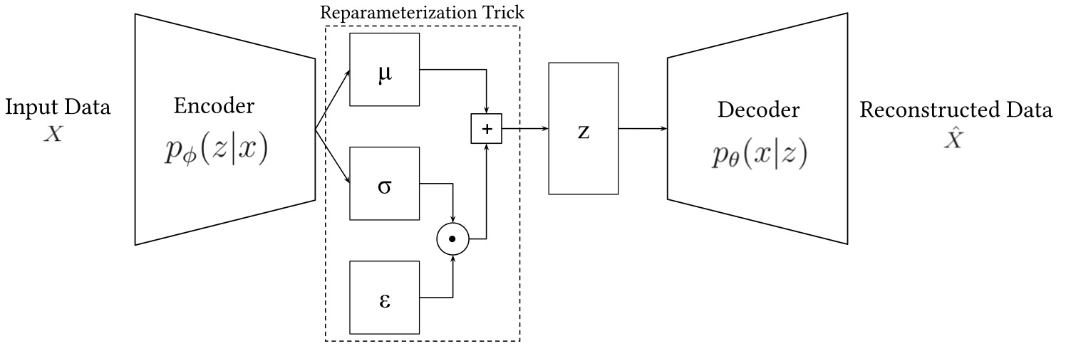
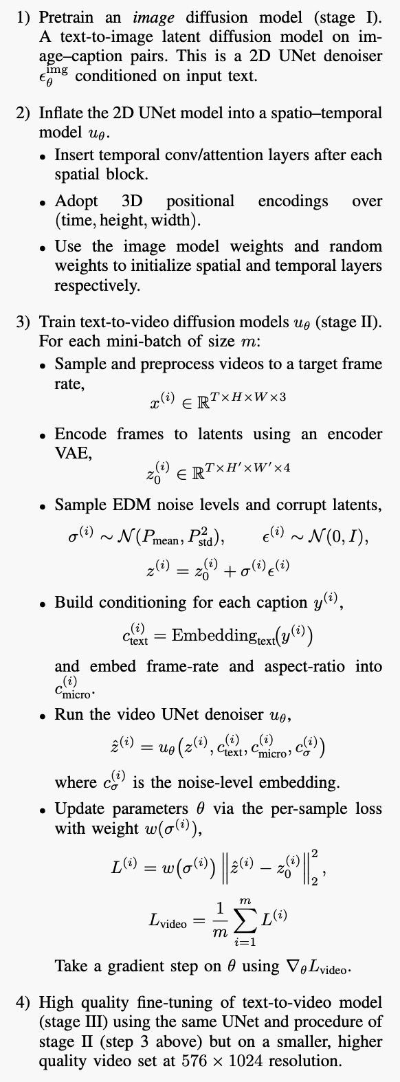
Autoencoders work by compressing the input data into a representation called latent space and reconstructing the input from that representation. Variational Autoencoders improve this framework by imposing structure on the latent space. Instead of letting latent codes drift arbitrarily, VAEs use a Kullback–Leibler (KL) term to force the latent space to follow a particular distribution such as a Gaussian. Given model parameters, the goal is to maximize the likelihood of seeing the real data, but the exact marginal likelihood is intractable in high-dimensional space. VAEs therefore use an encoder network that gives a tractable approximation of the latent posterior.
Below is the objective function for a VAE. The reconstruction term forces the decoder $p_\theta(x \mid z)$ to explain $x$ well when $z$ is sampled from the encoder $q_\phi(z \mid x)$. The regularizer $\mathrm{KL}(q_\phi(z \mid x)\,\|\,p(z))$ pushes the approximate posterior (encoder output) closer to the prior $p(z)$.
A key step that made VAEs practical was the reparameterization trick. It moves the randomness out of the neural network parameters and expresses the latent variable as a differentiable function of the mean, variance, and fixed Gaussian noise. This leads to much lower variance and makes end-to-end backpropagation possible.
Diagram of a Variational Autoencoder
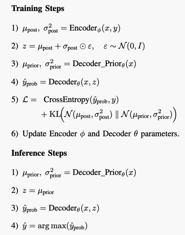
Below is a simplified illustration of the training process for a conditional VAE.
Simplified Training and Inference Procedure for the Conditional VAE
VAEs also introduced important failure modes. KL collapse, also known as posterior collapse, happens when the model stops encoding useful information about the input and the decoder learns to reconstruct without using the latent variable. Vanilla VAEs can also produce blurry reconstructions because a Gaussian decoder tends to converge toward the mean of the pixels. Conditional VAEs extended the framework by conditioning the generated output on the input, making VAEs useful for tasks such as image-to-image generation and structured prediction.
Later, several variants of VAEs tried to improve the original formulation. IWAE used a tighter log-likelihood lower bound through importance weighting. DRAW combined a recurrent VAE with a spatial attention mechanism so that the model could go from coarse to fine image pixels. VQ-VAE introduced a learned discrete codebook, resulting in sharper reconstructions and a learned prior rather than a fixed Gaussian. Deep hierarchical VAEs increased expressiveness by organizing the latent space into multiple levels so that high-level latents could guide finer latents.
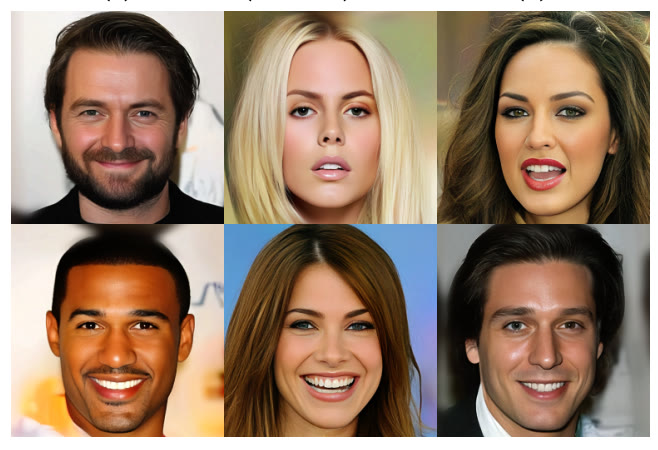
Sample Images Generated by NVAE[1]
Overall, VAEs provided a probabilistic framework for generative modeling through a tractable loss function that allows one to pass gradients through stochastic layers. They offered a strong probabilistic foundation, interpretability, and controllability, but they also suffered from an approximate likelihood objective, posterior collapse, and blurry reconstructions.
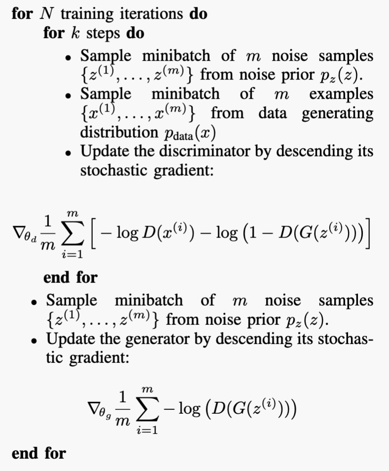
Generative Adversarial Networks
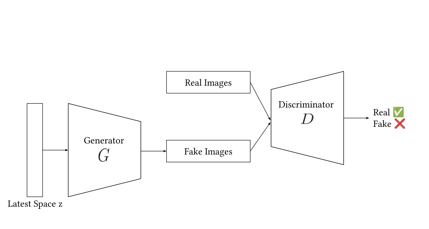
Generative Adversarial Networks were introduced shortly after VAEs. Their approach uses two models: a generator and a discriminator. The goal of the generator is to capture the data distribution by generating images that resemble the training data, and the goal of the discriminator is to discriminate whether a sample came from the training data or from the generator. This adversarial game provides a training signal for the generator through the discriminator’s gradient. One of the major advantages of GANs is that the whole network is trained end-to-end using backpropagation.
Overall GAN Architecture
Generator (G) and Discriminator (D) are trained simultaneously in a minimax game:
Below shows the simplified training procedure for a GAN-based model:
Simplified Training Procedure for a GAN
Later, DCGAN introduced a set of architectural changes that offered more stable training. It replaced pooling with strided convolutions, used batch normalization, and relied on deep convolutional layers instead of fully connected layers. These changes became foundational for later GAN work and produced cleaner samples than the earliest GAN results.
A major challenge in working with GANs is achieving stable and reliable training. As the discriminator gets better, the updates to the generator can deteriorate. This motivated a large body of work on training stability, including virtual batch normalization, minibatch discrimination, Wasserstein GAN, WGAN-GP, and zero-centered gradient penalties such as the R1 penalty. These methods tried to prevent vanishing gradients, mode collapse, and unstable two-player dynamics.
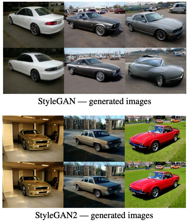
Conditional GANs extended the framework by feeding labels or other side information to both the generator and discriminator. Auxiliary Classifier GANs added an explicit class-prediction head and improved conditional image synthesis. Later, high-quality image generation advanced rapidly. Progressive Growing of GANs started with very low-resolution images and increased network complexity and image size progressively during training. StyleGAN mapped the latent code into an intermediate latent space, where early layers set the pose and shape and later layers determined color and fine details. StyleGAN2 reduced artifacts and improved training, while StyleGAN3 addressed texture sticking by incorporating anti-aliasing techniques inside the generator. Below shows sample images generated by StyleGAN and StyleGAN2.
Sample Images Generated by StyleGAN and StyleGAN2[2]
GANs also expanded beyond unconditional image synthesis. StackGAN showed how text embeddings could be used to synthesize high-quality images from text descriptions through a two-stage pipeline in which the second stage refined the coarse output of the first.
GANs had a long-lasting impact on image generation. They created the first photorealistic images and dramatically improved image quality over several years, but hard optimization, instability, and mode collapse remained recurring issues.
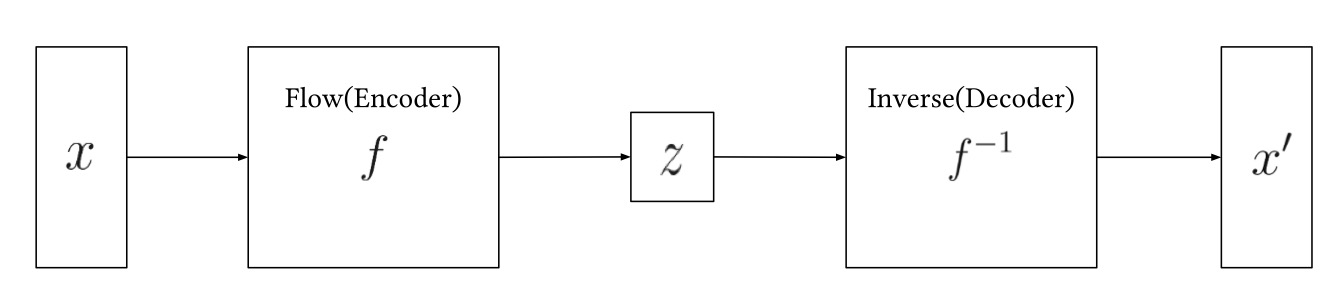
Normalizing Flows
The general idea behind normalizing flows is to transform data to a simple distribution, such as a Gaussian, via an invertible mapping without losing information. A sequence of reversible transformations maps the input into a latent space with a tractable density, making exact likelihood computation possible through the change-of-variable formula. This gave normalizing flows a strong mathematical foundation for image generation.
Simplified Normalizing Flows Architecture
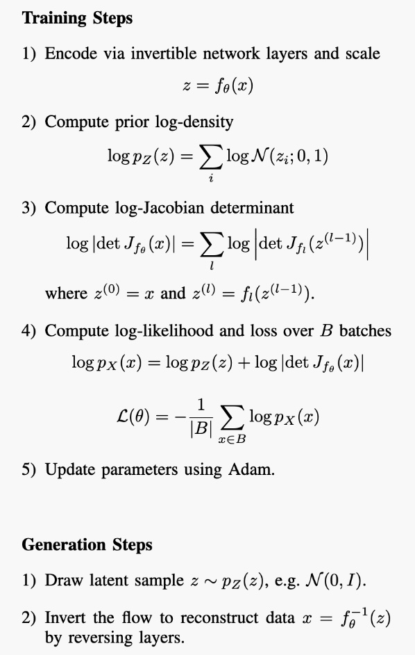
The exact log likelihood of normalizing flow can be computed via equation below where $J_{f_\theta}(x)$ is the Jacobian of the transformation $f_\theta$.
Below shows the simplified training and inference steps for a normalizing flow.
Simplified Training and Generation Steps for a Normalizing Flow
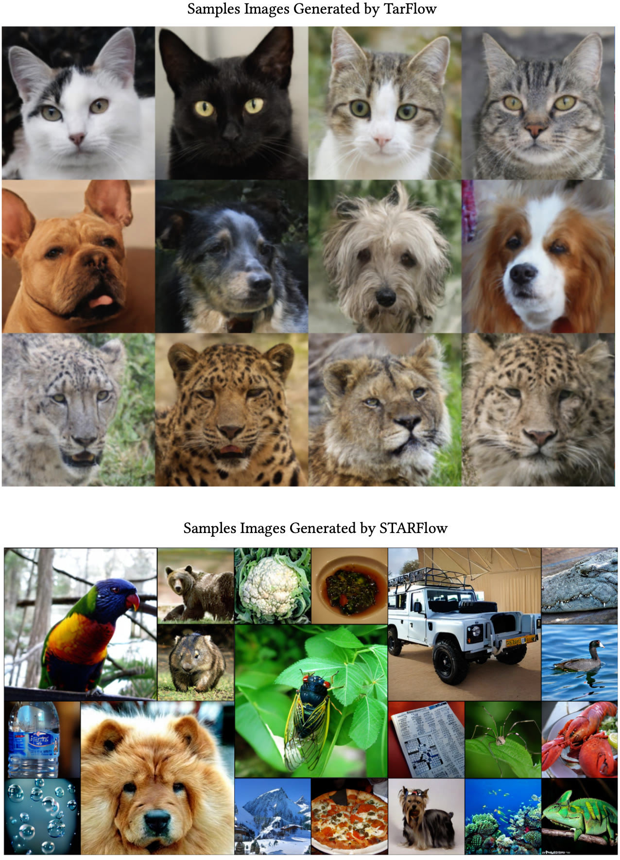
Later work used flows to improve the expressiveness of the posterior distribution in VAEs by passing a base density through a sequence of invertible maps. More modern perspectives showed that, under reasonable conditions, normalizing flows can represent very rich distributions and offer a unifying view of generative modeling and density estimation. Below shows sample images generated by Tarflow and Starflow.
TARFLOW[3] (top) and STARFLOW[4] (bottom) improve generation capabilities of Normalizing Flows.
Normalizing flows offer a simple but powerful formulation, exact likelihood, and one-step sampling. Their invertible formulation also makes it possible to inspect how latent changes affect pixels. At the same time, they struggle to model complex image generation tasks as well as diffusion and autoregressive models.
Transformer and Autoregressive Models
Autoregressive image generation models make predictions one token at a time. Early models achieved this with recurrent or convolutional networks, while later architectures adopted transformers. All of them follow the same next-token or next-patch prediction principle: generation conditions on everything produced so far as shown in the equation below.
\[p(\mathbf{x}) = \prod_{t=1}^{T} p(x_t \mid x_{<t}), \quad \text{where } T = H \times W \times 3\]
PixelRNN and PixelCNN were among the early autoregressive models that sequentially predicted pixels in raster order. PixelRNN used LSTMs to model dependencies across previously generated pixels, while PixelCNN used masked convolutions to provide more parallelization during training. Gated PixelCNN improved PixelCNN by introducing gating and removing blind spots in masked convolution. PixelCNN++ simplified the output distribution and improved optimization, and PixelSNAIL combined causal convolution with self-attention to better capture long-range dependencies.
After the Transformer architecture was introduced, it was adapted for autoregressive image generation. Image Transformer used self-attention over image blocks to predict the next pixels. iGPT treated images as token sequences and trained a transformer to autoregressively predict pixels, showing that large-scale autoregressive pretraining could learn useful visual representations.
Box below shows the training procedure for an autoregressive image transformer.
Simplified Training and Generation Steps for an Autoregressive Image Transformer
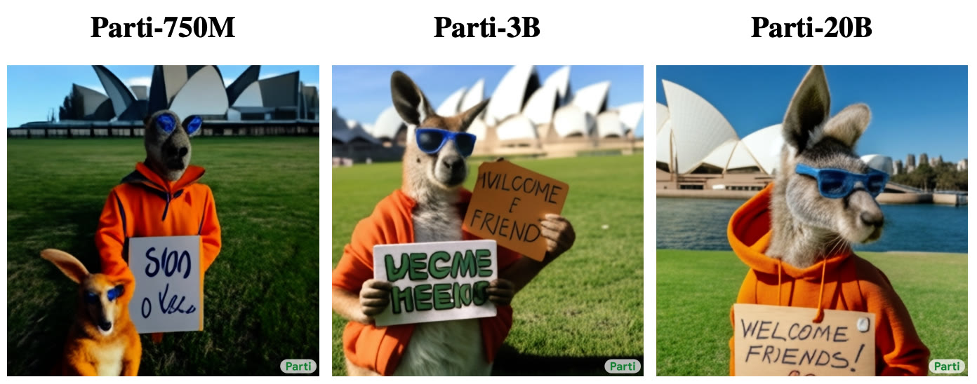
Scaling up text-to-image transformers required moving away from raw pixels. DALL-E 1 used a two-stage pipeline in which a VQ-VAE compressed an image into discrete tokens and an autoregressive transformer modeled the joint distribution of text tokens and image tokens. Related work replaced the VAE with VQGAN for high-resolution image synthesis. These approaches allowed transformers to model global structure while relying on learned visual tokens instead of raw pixels. Below shows sample images generated by a model called Parti[5] in which the authors used combinations of VQ-GAN and autoregressive transformers.
Improved sample quality in Parti[5] as the number of parameters in the autoregressive encoder–decoder increases from 750M to 20B.
Autoregressive models are among the most stable models when it comes to training and they are a great fit for conditional generation. Their main drawback is that generation can be slow and expensive because images are produced token by token.
Diffusion Based Models
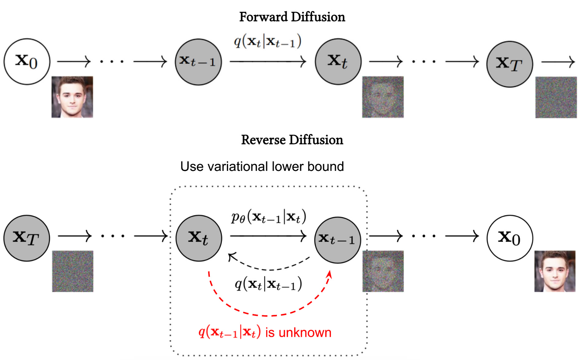
Diffusion models draw inspiration from physics and learn to reverse a stochastic diffusion process in which Gaussian noise is gradually added to an image until the image becomes nearly indistinguishable from isotropic Gaussian noise.
$$
x_t = \sqrt{\bar{\alpha}_t}\, x_0 + \sqrt{1 - \bar{\alpha}_t}\,\varepsilon,
\qquad
\varepsilon \sim \mathcal{N}(0, I)
$$
The goal of the model is to learn the reverse process, transforming pure noise back into data. Below diagram shows the forward and reverse diffusion processes.
Top[6]: Systematically destroying the structure in the image by gradually adding noise to the image. Bottom[7]: Learned reverse diffusion process to restore the original
image.
Early diffusion work established a strong mathematical foundation, but it was the introduction of Denoising Diffusion Probabilistic Models (DDPM) that made diffusion-based image generation take off. Below shows the simplified training steps for a DDPM.
Simplified Training and Generation Steps for a Denoising Diffusion Probabilistic Model
DDPM reparameterized the reverse mean so that the network predicts the noise added in the forward process. This led to a simple mean squared error objective and paired naturally with a UNet-style architecture with downsampling, upsampling, and attention. From there, a series of improvements focused on efficiency. DDIM accelerated generation by changing the sampling procedure without retraining the model. Progressive distillation reduced the number of denoising steps by training a student model to imitate multiple teacher steps at once. Distribution Matching Distillation and consistency models pushed this even further toward very few-step or even one-step generation.
Conditional diffusion models made the framework practical for controlled generation. ADM improved the architecture and used classifier guidance to shift the reverse diffusion process toward a desired label. Classifier-free guidance removed the separate classifier and jointly trained conditional and unconditional models in a single network. GLIDE extended these ideas to text conditioning and showed that classifier-free guidance produces more realistic images than CLIP guidance. Later work also clarified the design space of diffusion models by separating the denoiser itself from choices about noise schedules, preconditioning, and sampling.
A major shift happened when diffusion moved into latent space. Instead of denoising pixels directly, latent diffusion models first trained an autoencoder and then ran diffusion on the lower-dimensional latent representation. This reduced cost while preserving image quality and enabled flexible conditioning through cross-attention. Diffusion Transformers (DiT) later replaced the usual UNet backbone with a vision-transformer style model that operates on latent patches, showing that increasing transformer capacity strongly improves FID scores. Palette showed that the same diffusion framework could unify image-to-image translation tasks such as colorization, inpainting, uncropping, and JPEG restoration.
Scaling up diffusion models led to many influential text-to-image systems. DALL-E 2 combined CLIP embeddings with a hierarchical diffusion pipeline. Imagen used a very large pretrained T5 model as the text encoder and a cascade of diffusion models to upsample from low resolution to high resolution. DALL-E 3 focused on prompt following by re-captioning the training data with a stronger captioner. Figure below shows the impact of re-captioning on the quality of the generated images. Stable Diffusion XL expanded the UNet, used richer text conditioning, and added a refinement model for high-resolution synthesis.
Top and bottom images show the original and upsampled image captions, respectively. Images generated by DALL-E 3. [8]
Diffusion models evolved from iterative pixel-domain denoising to faster latent-space denoising, from UNet backbones to transformer backbones, and from standalone research models to full product systems. Over time, they became a dominant choice for high-quality image generation.
Recent Developments in Image Generation
Many top image generation systems have shifted from classic diffusion-based formulations and moved toward Rectified Flow and Flow Matching, motivated by cleaner continuous-time dynamics, improved training stability at scale, and image generation in fewer sampling steps. In these models, generation is framed through an ordinary differential equation in which a learned vector field transports noise toward the data distribution.
Rectified Flow learns a causal drift field along a straight-line interpolation between noise and data. A key motivation is efficiency: if the trajectory from noise to image is straighter, the sampler can take larger steps and reach the final sample in fewer iterations. Reflow further straightens the trajectories and improves sampling efficiency. Later work scaled Rectified Flow to high-resolution text-to-image generation with transformer backbones and improved one-round training while keeping the number of function evaluations low. For training, they draw independent pairs $(X_0, X_1) \sim \pi_0 \times \pi_1$, and consider the straight line interpolation between endpoints,
$$
X_t = (1 - t)X_0 + tX_1,\qquad t \in [0,1]
$$
The corresponding velocity along this path is $X_1 - X_0$. However, this velocity is not causal at time $t$ because it depends on the unknown point $X_1$. Rectified Flow therefore fits a causal drift field $v_\theta(X_t,t)$ via:
$$
\hat{\theta} = \arg\min_{\theta}\,\mathbb{E}\left[\left\|(X_1 - X_0) - v_\theta\!\left((1 - t)X_0 + tX_1, t\right)\right\|^2\right]
$$
where $t \sim \mathrm{Uniform}([0,1])$.
Flow Matching also learns an ODE velocity field, but it provides a more general framework that matches a target probability path through conditional objectives. Depending on the chosen path, it can recover diffusion-style paths or optimal-transport-style paths. In practice, Flow Matching has shown improvements in sample quality, likelihood, and evaluation time relative to diffusion baselines. If we have a target probability path for the data distribution $p_t(x)$ and a vector field $u_t(x)$ that generates it, then Flow Matching (FM) trains a neural network $v_\theta(x,t)$ via regression:
$$
\mathcal{L}_{\mathrm{FM}}(\theta)=\mathbb{E}_{t\sim U[0,1],\,x\sim p_t}\left[\|v_\theta(x,t)-u_t(x)\|^2\right]
$$
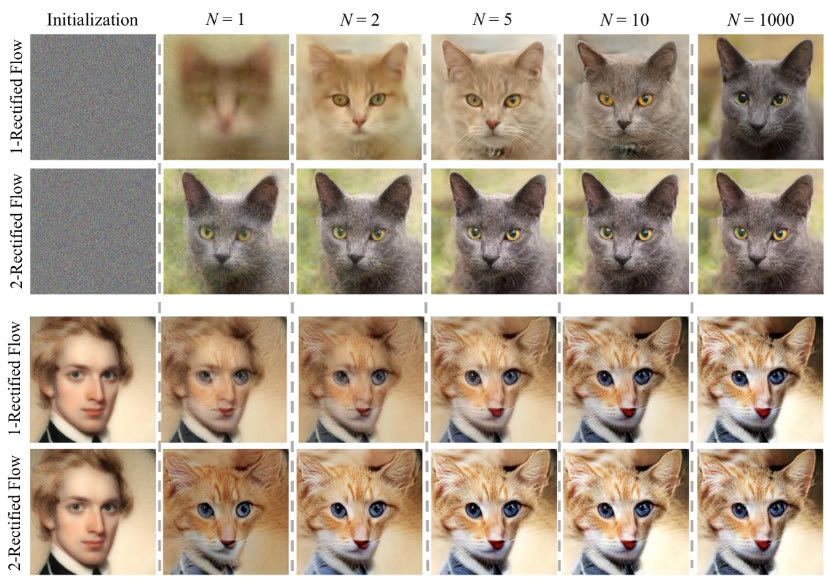
Figure below shows different rectified flow trajectories for image generation. The upper two rows show the mapping from noise to image, with the second row showing the impact of reflow. With reflow, fewer steps are needed to generate the final image. The lower two rows show a similar behavior but with image to image transport.
Rectified Flow[9] and reflow trajectories. The top two rows illustrate noise to image transport under Rectified Flow. The second row shows reflow that produces straighter paths that can be traversed with fewer numerical integration steps. The bottom rows show an analogous effect for image to image transport, where reflow similarly reduces curvature and improves sampling efficiency.
Rectified Flow and Flow Matching provide new objectives and a new framework for designing the next generation of image generation systems. Looking at these modern architectures, one can see that they often consist of a stack of text conditioning, transformer backbones, and increasingly efficient sampling techniques.
Video Generation
Video generation can be formulated as image generation expanded over time while keeping temporal consistency across frames. As image generation models improved, researchers started to transfer the same ideas to the video domain.
Early work extended GANs to video. VideoGAN modeled the stationary world and moving objects with a two-stream architecture consisting of foreground, background, and a learned mask. This allowed the model to capture coarse motion patterns while separating static and dynamic content.
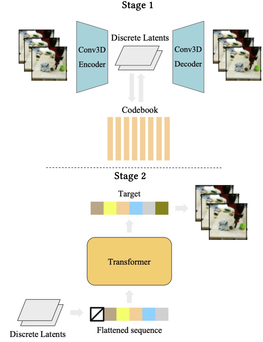
Transformer-based video generation built on discrete latent representations. A standard VQ-VAE first learned discrete video latents, and an autoregressive transformer was then trained over the flattened spatiotemporal token sequence. This mirrored the token-based autoregressive approaches used in images. Below diagram shows the two stage training pipeline for VideoGPT[10]. In stage 1, the VQ-VAE is trained and in stage 2 a GPT-style transformer is trained over latent codebooks.
Two stage training pipeline for VideoGPT. In stage 1, the VQ-VAE is trained and in stage 2 a GPT-style transformer is trained over latent codebooks.
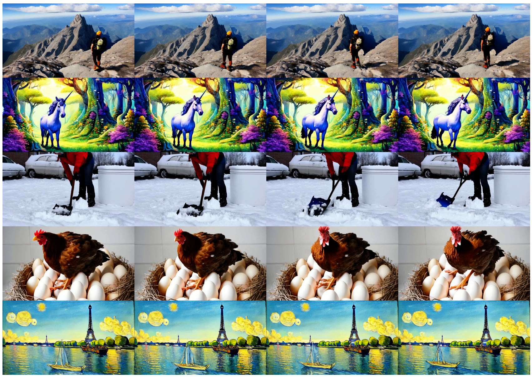
Diffusion-based video generation trained a diffusion model that directly modeled blocks of frames as a single object. The main architectural change was a 3D UNet denoiser that processed space and time jointly. Later work scaled latent video diffusion models through stronger image pretraining, larger datasets, and improved training strategy. Stable Video Diffusion was one of the first widely used open-source latent video diffusion models and showed the importance of image pretraining for human preference. Below shows the training steps for Stable Video Diffusion.
Training steps for Stable Video Diffusion[11]. The model is trained on latent video representations using a 3D UNet denoiser.
Below shows sample frames generated by Stable Video Diffusion with different text prompts.
Text-to-video samples from the stable video diffusion (SVD)[11] model. Captions from top to bottom are: “A hiker is reaching the summit of a mountain, taking in the breathtaking panoramic view of nature.”, “A unicorn in a magical grove, extremely detailed.”, “Shoveling snow”, “A beautiful fluffy domestic hen sitting on white eggs in a brown nest, eggs are under the hen.”, and “A boat sailing leisurely along the Seine River with the Eiffel Tower in background by Vincent van Gogh”.
The foundation of video generation still relies on the same core ideas as image generation: strong pretraining, diffusion as an efficient representation, and large-scale data. Active research areas include long-range temporal coherence, physical causality, fine detail, and compute efficiency.
Fake Image Generation and Societal Impacts
As image generation models improve, there is growing concern about their use. The risks include fake photos or videos of public figures, images that closely mimic the style of another artist, harmful and unfair representations of people and cultures, pressure on artists and creators, phishing through fake receipts or proof, and creating fake images of someone without permission. As generated images become increasingly difficult to distinguish from real images, their potential misuse can have increasingly severe impacts.
Given these concerns, many efforts have gone into image manipulation detection. Earlier work detected duplicated regions and other statistical inconsistencies left behind by digital editing. Later research on face manipulation showed how realistic reenactment and audio-driven talking faces could be produced, which in turn increased the urgency of detection work.
Deepfake detection methods analyzed temporal cues such as eye blinking and benchmarked face-video forensics under more realistic conditions. Other work showed that GAN-generated images leave behind artifacts in the frequency domain because convolutional upsampling introduces systematic spectral distortions. These artifacts can be exploited to classify real versus generated images.
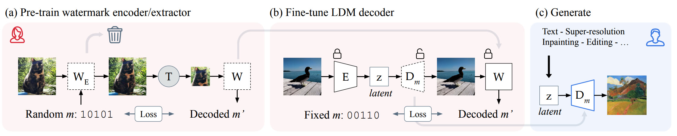
As diffusion models made generated images more realistic, detection became harder. This motivated watermarking and inversion-based techniques that exploit the reconstruction path of diffusion-generated images. Below shows an example of the stable signature steps used for watermarking diffusion-generated images.
Stable signature[12] steps. (a) Pre-training the watermark encoder and decoder. (b) Finetuning the diffusion decoder. (c) Generating an image with invisible watermarks.
Recent empirical scaling trends suggest continued improvements in the capabilities of these models. A central challenge is establishing effective safeguards against potential misuses. Do we have adequate safety measures in place? Are we prepared for a future in which the harmful uses of image generation systems, described above, are realized at scale? Given the risks associated with these powerful image and video generation models, we need both technical and societal solutions to mitigate these risks and to ensure preparedness for worst case scenarios.
Conclusion
Image generation models have gone through a revolution in the past decade. We started from models that were able to generate low quality images in a restricted setting to today's models that are able to generate images with exceptional quality and user control. Users can control different aspects of the generated images including quality, fine details, style, background, coloring, etc.
VAEs provided a probabilistic framework for generative image modeling. They are still valuable when interpretability and controllability of the generated output matter. GANs had probably the most impact by creating the first photorealistic images; however, mode collapse and instability of training were recurring issues with them.
Normalizing flows offered a simple but powerful mathematical framework for image generation. Their invertible formulation, exact likelihood, and one-step sampling made them an excellent candidate for image generation; however, they struggle to model complex image generation tasks as well as diffusion and autoregressive models. Autoregressive models are among the most stable models when it comes to training. They are also a great fit for conditional generation because of their autoregressive nature, but this autoregressive nature comes with a price, since generation can be slow and expensive.
Diffusion models started from iterative pixel domain denoising and evolved to faster, few iteration latent space denoising. The overall complexity of diffusion model architectures increased as their capabilities grew. Architectural advances enabled conditioning on other modalities such as text and image embeddings.
Rectified Flow and Flow Matching provide new objectives, as well as a new framework for designing the next generation of image generation systems. These include defining a transport path, a learned vector field, and a new sampling pipeline with as few function evaluations as possible.
Finally, as image generation models become more capable, the potential misuses (deepfakes, fraud, manipulation, privacy harm) of these models become easier to scale. As a result, safety measures are critical when deploying these models. Moving forward, there are still areas that require further progress. These include efficient generation in fewer diffusion steps, better temporal and 3D consistency, strong conditioning to users' input, watermarking, and responsible usage.
To Cite this work
@article{shirvani2026image,title={Image Generation Models: A Technical History},author={Shirvani, Rouzbeh},journal={arXiv preprint arXiv:2603.07455},year={2026}}
Acknowledgements
Thanks to Sean McGregor for help with publishing the paper.
🎉 Thanks for subscribing!
References
Vahdat, A. and Kautz, J.: "NVAE: A Deep Hierarchical Variational Autoencoder", NeurIPS 2020; arXiv:2007.03898.
Karras, T., Laine, S., Aittala, M., Hellsten, J., Lehtinen, J., and Aila, T.: "Analyzing and Improving the Image Quality of StyleGAN", CVPR 2020; arXiv:1912.04958.
Zhai, S., Zhang, R., Nakkiran, P., Berthelot, D., Gu, J., Zheng, H., Chen, T., Bautista, M. A., and others: "Normalizing Flows are Capable Generative Models", ICML 2025; arXiv:2412.06329.
Gu, J., Chen, T., Berthelot, D., Zheng, H., Wang, Y., Zhang, R., Dinh, L., Bautista, M. A., and others: "STARFlow: Scaling Latent Normalizing Flows for High-resolution Image Synthesis", 2025; arXiv:2506.06276.
Yu, J., Xu, Y., Koh, J. Y., Luong, T., Baid, G., Wang, Z., Vasudevan, V., Ku, A., Yang, Y., Ayan, B. K., and others: "Scaling Autoregressive Models for Content-Rich Text-to-Image Generation", arXiv preprint 2022; arXiv:2206.10789.
Ho, J., Jain, A., and Abbeel, P.: "Denoising Diffusion Probabilistic Models", Advances in Neural Information Processing Systems, vol. 33, pp. 6840-6851, 2020; arXiv:2006.11239.
Liu, X., Gong, C., and Liu, Q.: "Flow Straight and Fast: Learning to Generate and Transfer Data with Rectified Flow", arXiv preprint 2022; arXiv:2209.03003.
Yan, W., Zhang, Y., Abbeel, P., and Srinivas, A.: "VideoGPT: Video Generation Using VQ-VAE and Transformers", arXiv preprint 2021; arXiv:2104.10157.
Blattmann, A., Dockhorn, T., Kulal, S., Mendelevitch, D., Kilian, M., Lorenz, D., Levi, Y., English, Z., Voleti, V., Letts, A., and others: "Stable Video Diffusion: Scaling Latent Video Diffusion Models to Large Datasets", arXiv preprint 2023; arXiv:2311.15127.
Fernandez, P., Couairon, G., Jégou, H., Douze, M., and Furon, T.: "The Stable Signature: Rooting Watermarks in Latent Diffusion Models", Proceedings of the IEEE/CVF International Conference on Computer Vision, pp. 22466-22477, 2023; arXiv:2303.15435.
🎉 Thanks for subscribing!
I would love to hear your
thoughts in the comments below.